translation | Math in Matter

Ehrenfest theorem allows us to see how physical quantities evolve through time in terms of other physical quantities. In quantum mechanics, physical quantities, like momentum or position, are represented by operators. To get the average value of a physical quantity of a system, we act the operator on a wavefunction. The wavefunction represents the physical system’s probabilistic behavior. The average of a physical quantity is called an “expectation value”.

The expectation value of an operator $\mathscr{O}$ is:
$\left< \mathscr{O} \right> = \left< \Psi \left| \mathscr{O} \right| \Psi \right> = \int dx \Psi^{\dagger} \mathscr{O} \Psi$
where $\Psi$ is a wavefunction $\Psi(x)$ .

This definition allows us to take a time derivative of the expectation value.
$\frac{d}{dt}\left< \mathscr{O} \right> = \frac{d}{dt} \left< \Psi \left| \mathscr{O} \right| \Psi \right> = \frac{d}{dt} \int dx \Psi^{\dagger} \mathscr{O} \Psi$
The total derivative moves inside the integral as a partial derivative, where we use the product rule to differentiate:
$= \int dx (\frac{\partial}{\partial t} \Psi^{\dagger} \mathscr{O} \Psi + \Psi^{\dagger} \frac{\partial}{\partial t} \mathscr{O} \Psi + \Psi^{\dagger} \mathscr{O} \frac{\partial}{\partial t} \Psi)$

A time derivative acting on a wave function is equivalent to a Hamiltonian operator acting on a wave function (with a factor of $\frac{1}{i \hbar}$ ):
$\frac{\partial}{\partial t} \Psi = \frac{1}{i \hbar} H \Psi$
Take the complex conjugate:
$\frac{\partial}{\partial t} \Psi^{\dagger} = \frac{-1}{i \hbar} \Psi^{\dagger} H$

We can then swap the time derivatives for Hamiltonians:
$\frac{d}{dt}\left< \mathscr{O} \right> = \int dx ( \frac{-1}{i \hbar} \Psi^{\dagger} H \mathscr{O} \Psi + \Psi^{\dagger} \frac{\partial}{\partial t} \mathscr{O} \Psi + \frac{1}{i \hbar} \Psi^{\dagger} \mathscr{O} H \Psi)$
$= \frac{-1}{i \hbar} \left< \Psi \left| H \mathscr{O} \right| \Psi \right> + \left< \Psi \left| \frac{\partial}{\partial t} \mathscr{O} \right| \Psi \right> + \frac{1}{i \hbar} \left< \Psi \left| \mathscr{O} H \right| \Psi \right>$
The first and last terms can be combined using a commutator:
$= \left< \Psi \left| \frac{\partial}{\partial t} \mathscr{O} \right| \Psi \right> + \frac{1}{i \hbar} \left< \Psi \left| [\mathscr{O},H] \right| \Psi \right>$

So then we have Ehrenfest Theorem, relating the time derivative of an expectation value to the expectation value of a time derivative:
$\frac{d}{dt}\left< \mathscr{O} \right> = \left< \frac{\partial}{\partial t} \mathscr{O} \right> + \frac{1}{i\hbar}\left< [\mathscr{O},H] \right>$

The general form of the Hamiltonian $H$ , has a momentum-dependent kinetic energy term, and a position-dependent potential energy term $V(x)$ .
$H = \frac{p^2}{2m} + V(x)$

As an example, let’s see how changes in momentum over time can be expressed.
$\frac{d}{dt}\left = \left< \frac{\partial}{\partial t} p \right> + \frac{1}{i\hbar}\left< [p,H] \right>$
Momentum doesn’t have an explicit time-dependence, so the first term is zero. Further, operators commute with themselves: $[p,p^2] = 0$ , so the Hamiltonian reduces to just the potential energy term. So we’re left with:
$\frac{d}{dt}\left = \frac{1}{i\hbar}\left< [p,V(x)] \right>$

To see what this remaining commutator of operators reduces to, we will have to use a little calculus. Momentum expressed in terms of position is essentially the derivative operator:
$p = -i\hbar \frac{d}{dx}$ . Keep in mind that potential energy is a function of position which is why momentum does not commute with it.
Since we are dealing with operators, we need them to act on something: we’ll use a dummy wavefunction $\Phi(x)$ . Then just remember the product rule for derivatives:
$[p,V]\Phi = -i\hbar[\frac{d}{dx},V]\Phi = -i\hbar(\frac{d}{dx}V\Phi - V\frac{d}{dx}\Phi) = -i\hbar(\frac{d}{dx}V)\Phi$
So then we can see that the change in the expectation value of momentum with respect to time is:
$\frac{d}{dt}\left =-\left< \frac{d}{dx}V(x) \right>$
On the left you have impulse over change in time, and on the right you have change in potential energy over change is position. Both are ways of measuring force in classical physics. In fact, this Newton’s second law!
$\frac{d}{dt}\left = \left< F \right>$

If we do the same for change in expectation value of position with respect to time, we get an equation for velocity:
$\frac{d}{dt}\left< x \right> = \left< \frac{\partial}{\partial t} x \right> + \frac{1}{i\hbar}\left< [x,H] \right>$
Again, position has no explicit time-dependence, so the first term is zero. However, now position commutes with potential energy (since it’s just a function of position), and position does not commute with kinetic energy (momentum). So we’re left with:
$\frac{d}{dt}\left< x \right> = \frac{1}{i\hbar} \frac{1}{2m}\left< [x,p^2] \right>$
If we go through the dummy wavefunction process we’ll arrive at:
$\frac{d}{dt}\left< x \right> = \frac{\left}{m}$
which is the classical definition of velocity.

In algebra, or pre-calc, you learn that you can change the position of a function by modifying the argument. In quantum physics this idea is used to displace wave functions. If a function starts off at one position, and moves to another position, all that is needed is a change in argument. However, quantum physics likes to use linear operators to alter functions. What would an operator look like if it can change the argument of a function? In this post, I will construct a 1-D example of such an operator.

A general wave function can be written as: $\Psi (x)$ , where the shape of $\Psi$ is dependent on the spatial variable $x$ .
To translate a function by distance $a$ , modify the argument of $\Psi$ ,
To move the function right by $a$ , $\Psi(x) \rightarrow \Psi (x-a)$
To move the function left by $a$ , $\Psi(x) \rightarrow \Psi(x+a)$
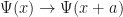
Let’s just take the $\Psi(x+a)$ example, and without loss of generality say that $a$ can be positive or negative.
Next we can take advantage of Taylor expansions.
A function $f(x)$ can be expanded around a point $a$ : $f(x) = f(a) + (x-a)\frac{d}{dx}f(a) + \frac{(x-a)^2}{2!} \frac{d^2}{dx^2}f(a) + ...$
Here, in our example, we want to expand $\Psi(x+a)$ around $x$ , to express the translated function $\Psi(x+a)$ in terms of the original function $\Psi(x)$ :
$\Psi(x+a) = \Psi(x) + a\frac{d}{dx}\Psi(x) + \frac{a^2}{2!} \frac{d^2}{dx^2} \Psi(x) + ...$
Note: $\frac{d}{dx} = \frac{i}{\hbar} p$ .
A more complete version of this expression would be:
$\Psi(x+a) = \sum\limits_{n=0}^{\infty} \frac{a^n}{n!} \frac{d^n}{dx^n} \Psi(x) = \Psi(x) + \sum\limits_{n=1}^{\infty} \frac{a^n}{n!} \frac{d^n}{dx^n} \Psi(x)$
This sum’s structure is similar to the Taylor expansion of the exponential function.
$e^x = 1 + x + x^2/2! + ... = \sum\limits_{n=1}^{\infty} \frac{x^n}{n!}$
Every operator in the $\Psi(x+a)$ expansion can be reduced into an simplified operator: $\Psi(x+a) = e^{a\frac{d}{dx}} \Psi(x)$
$= e^{\frac{ai}{\hbar} p} \Psi(x)$ .
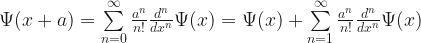
This new operator $e^{a\frac{d}{dx}}$ can be expanded to return to what we had before: $e^{a\frac{d}{dx}} = \sum\limits_{n=0}^{\infty} \frac{a^n}{n!} \frac{d^n}{dx^n}$ .
So the translated function is a version of the original function with a specific type of interference. Such that the structure is: $Translated = Original + Interference$ .
$\Psi(x+a) = \Psi(x) + \sum\limits_{n=1}^{\infty} \frac{a^n}{n!} \frac{d^n}{dx^n} \Psi(x) = \Psi(x) + \Delta(a)\Psi(x)$
We can reduce the operators in the interference terms into an exponential in the usual way:
$\Delta(a) = \sum\limits_{n=1}^{\infty} \frac{a^n}{n!} \frac{d^n}{dx^n}$
$= e^{a \frac{d}{dx} } - 1$

The expectation value $\left< e^{a\frac{d}{dx}} \right>$ characterizes the average overlap between $\Psi(x)$ and $\Psi(x+a)$ .
$\left< e^{a\frac{d}{dx}} \right> = \left< \Psi(x) \right| e^{a\frac{d}{dx}} \left| \Psi(x) \right>$
$= \left< \Psi(x) | \Psi(x+a) \right>$
$= \left< \Psi(x) \right| 1 + \Delta(a) \left| \Psi(x) \right>$
$= 1 + \left< \Delta(a) \right>$
The expectation value of the translation operator is then unity plus the expectation value of the interference operator.
$\left< \Delta (a) \right> = \sum\limits_{n=1}^{\infty} \frac{a^n}{n!} \left< \frac{d^n}{dx^n} \right>$
$= \sum\limits_{n=1}^{\infty} \frac{(ia)^n}{(\hbar)^n n!} \left< p^n \right>$
The interference expectation value is shown to be an expectation value of a function of the momentum operator.
In the case of localized waves, as $a$ gets much greater than the width of $\Psi(x)$ , the interference term approaches -1, since the overlap between the original and translated wave function decreases. This is equivalent to the original and displaced wave function becoming more and more orthogonal.
limit $_{a\rightarrow \infty} \left< \Delta (a) \right> = -1$
limit $_{a\rightarrow \infty} \left< \Psi(x) | \Psi(x+a) \right> = 0$