The planets and other bodies in our solar system orbit the sun along elliptical trajectories. For a given body, its elliptical orbit has the sun located at one of the two foci. For most of the planets, the eccentricity of their orbits is low, so they are approximately circular, and other bodies like comets have high eccentricity. This still begs the question: how are stable orbits asymmetric if the gravitational field from the sun is spherically symmetric? The reason is the periodic exchange of energy between kinetic and potential. You see this phenomenon occur in a pendulum or a spring. As these objects oscillate, energy is changing form while the total remains constant (neglecting friction). In a perfectly circular orbit, however, there is no exchange, since kinetic and potential energy each remain constant.
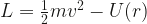
The physics of this can be worked out using Lagrangian mechanics. The first step is writing a Lagrangian describing an orbiting body. This is composed of the kinetic and potential energy of the body. The kinetic energy is dependent on its velocity. The potential energy is dependent on its distance from the sun. These can be put together to give us the Lagrangian : where is the velocity of the planet, is the mass of the planet, and is the potential energy from the sun’s gravity, which is dependent on radial distance . The explicit form of is not relevant yet.
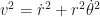
It is easier to work in polar coordinates rather than Cartesian coordinates for this problem. We can simplify things by noting that the planet is not leaving the plane of its orbit. So the coordinate is zero. Then the and coordinates can be converted to polar coordinates and . Take the derivative with respect to time to get the velocity vector, and then square it for the kinetic energy term. We are then left with a Lagrangian in polar coordinates:
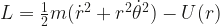
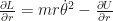
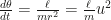
There are two degrees of freedom here: radial and angular. To get the equations of motion, we need to evaluate the Euler-Lagrange equation for each degree of freedom. For angular: since there is no explicit dependence on angle . This variable is a constant with respect to time, and is the angular momentum of the orbiting body. We can then express the equation of angular velocity in terms of :
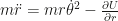
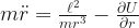
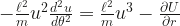
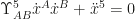
For the radial degree of freedom: Equate these together and you get the equation of motion: Plug in the equation for angular velocity, and the equation of motion only depends on : This differential equation can then be solved to get the trajectory of an orbiting body.
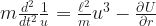
To solve this differential equation, do a change of variables: distance to inverse distance such that: We then have:
Because there is no explicit dependence on angle in the Lagrangian, time dependence can be converted to angular dependence.
The equation of motion then becomes:
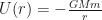
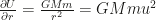
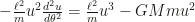
We now need the explicit form of the potential energy from the sun’s gravity to continue solving this. The equation is: Where is Newton’s constant and is the mass of the sun.
The equation of motion can then be simplified further:
Solving this is relatively easy with a variable substitution: The general solution is then: However, without loss of generality, this can be expressed with just one trigonometric function. Note that:
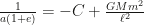
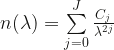
So now we have the general solution: The constant can be shown to be equal to . where is the eccentricity of the trajectory, not Euler’s number. Put back in terms of distance, we have a function for a trajectory in terms of angle and radial distance:
Note that different values of eccentricity give different trajectory shapes: Circle Ellipse Parabola Hyperbola Each of these is a conic section: a 2D cross-section of a 3D cone.
For simplicity, we can choose an axis where such that . So then we have:
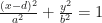
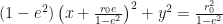
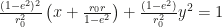
We can verify that this trajectory is a conic section by transforming it into Cartesian coordinates to look something like this:
Here the transformation is done step by step: The last step is then putting the trajectory equation into the form shown above. Where the variables here and relate to the variables , and : So the trajectory can be written in terms of and : Or back in polar coordinates:
A bound orbit with has a min and max distance from the sun, a semi-major axis, and a semi-minor axis. semi-major axis semi-minor axis perihelion (minimum distance to sun) aphelion (maximum distance to sun) Using this is actually how you solve for the constant in the general trajectory formula. For , we can say the planet is nearest to the sun, so , and for , we can say it is at its farthest from the sun, so . This gives a system of two equations that can be solved:
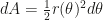
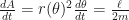
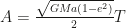
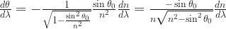
From here, we can arrive at Kepler’s law of equal areas. This is the observation that an orbiting body sweeps out the same area between it and the sun for any given duration of time. Start with an infinitesimal piece of swept area: Divide by an infinitesimal piece of time: And there you have it, the rate of the area swept over time is constant. We can express this constant in terms of the semi-major axis, and arrive at another of Kepler’s laws relating the orbital period to the semi-major axis. The full orbit area and period are then related by: The area of the ellipse in terms of the semi-major axis is: So we then have the law relating the orbital period with the semi-major axis:
Take the log of both sides, and we can see how planets and other objects fall on the curve.
The orbital period and semi-major axis of the planets were gathered from Wikipedia. However, if you were to measure these quantities yourself, you could use regression to check Kepler’s law and measure the mass of the sun. From the numbers given in Wikipedia, we compute the ratio between exponents on the period and semi-major axis to be and the mass of the sun to be .
This entry is for those who may be taking a symbolic logic or Boolean algebra course and find it hard to keep track of things. Symbolic logic has an abundance of symbols representing logical operations, or conjunctions, between premises to form statements or arguments. The symbols you are likely to see are listed below with the generic premises P and Q: Not P P and Q P or Q (inclusive or) If P then Q P If and only if Q P xor Q (exclusive or)
In addition to keeping track of several symbols, you have to remember the corresponding truth tables. The premises P and Q can both be either true T or false F, and the truth value of an argument consisting of the conjunction of P and Q is typically represented in a truth table which lists all the combinations of values and the resulting argument values.
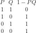
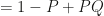
For example, the truth table for “P and Q” is:
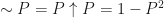
When I took the class, I wondered if there was a more succinct way to capture the structure of these operations. All arguments can be constructed in terms of “and”, “inclusive or” and “not” operations. Even the “if-then”, “if-and-only-if”, and “exlusive or” can be written in terms of “and”, “inclusive or” and “not”. The reduction does not have to stop there. All statements can be constructed in terms of “nand” (not-and). The symbol for this is the Sheffer stroke . P nand Q The other operations can be worked out in terms of nand: Not P P and Q P or Q
However, I felt like this removes a lot of the intuition. So I present another approach here. The nand operation can be expressed in terms of arithmetic operations if true and false are mapped to 1 and 0, respectively: and
The continuous surface aligns with the discrete logic points.
This isn’t a unique arithmetic representation, since there are other formulas that can represent nand, but this one seems like the simplest.
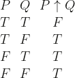
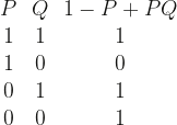
The truth table for “P nand Q” is:
Or rather, since and :
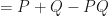
We can then work out the arithmetic formulae for each logical operation. For “not P” we have: Premises values are idempotent Therefore:
“P and Q” can be worked out the same way, by using the to replace all the Sheffer stroke operations with arithmetic.
P or Q :
If P then Q. (Note the asymmetry in the if-then truth table is represented in the formula.)
P if and only if Q:
By this point, you can use the above relations to replace other operators with arithmetic. For example, the exclusive or operation “P xor Q” can be expressed in terms of “or” and “and”:
To put it all together, here are the arithmetic formulae for logical operations: Not P P and Q P or Q P xor Q if P then Q P if and only if Q You can memorize these in place of truth tables.
In a previous blog entry, I show the “derivation” of the Schrödinger equation, which governs the behavior of the probabilistic wave function of a quantum particle. In this entry, I will show how this is related to the heat flow and temperature gradients we experience in our everyday lives.
Picture of me at Joseph Fourier’s grave in Père Lachaise Cemetery.
Deriving the Heat Equation
We have an intuitive understanding that heat flows from hot objects to colder objects nearby. This is the second law of thermodynamics. It also applies to a single object like a sheet of metal, a cooking pan, or a wire. If there is a spot on that object that is hotter than the rest of the object, perhaps from a heat source, heat from that spot will spread out through the object over time. Here I will derive the heat equation, which was developed by Joseph Fourier.
First, start with Fourier’s law of heat transfer, which is an experimental result. It models the relationship between heat conduction or flow rate in a material and the temperature gradient along the direction of heat flow through that material. Imagine we are dealing with a roughly 1-dimensional object like a wire. The law of heat transfer in that wire will be: Where: Is the heat flow. Is the temperature gradient along the wire length . Is the thermal conductivity of a material.
Visualization of heat flow through a segment of material.
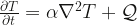
In the visualization above, the heat going into segment at is . The heat going out of segment at is Energy conservation (the first law of thermodynamics) demands the net amount of heat flow in the segment is the difference between the flow in (at ) and flow out (at ). Applying Fourier’s law of heat transfer to this equation we have: The amount of heat flowing in/out of the material will raise/lower its temperature according to the material’s mass and heat capacity . For a flow rate , a total amount of heat flows through after a time duration . Applying these substitutions to the energy conservation equation we have: Note that the material here is a wire, so we can consider a 1-D density : Doing some rearranging we have: Shrinking these differences to infinitesimal differences gives us a partial differential equation: namely the heat equation! With a heat source term we have: Note thermal diffusivity of the material here: This can be extended to include more dimensions to model how the temperature gradient changes as heat flows through a 2-d (plate) or 3-d (block) material.
Transformation
We can transform the Heat equation into the Schrödinger equation by making some variable substitutions. Both equations are partial differential equations with first-order derivatives with respect to time and second-order derivatives with respect to space. To perform this transformation follow the steps below: Turn temperature into quantum wave function (probability density) multiplied by Planck’s constant : So one can imagine quantum waves behaving like temperature. We can turn thermal diffusivity into quantum spin unit divided by mass : Turn the heat source term into the potential energy times the quantum wave function multiplied by : So this is interesting, it means the “heat source” is dependent on the “temperature”, which is distinct from what we encounter in our day-to-day. Turn time into imaginary time (This is known as a Wick rotation): The presence of imaginary numbers here implies oscillation. This is how real “temperature” becomes complex probability waves, with real and imaginary components. We then have the Schrödinger Equation:
1-D Case
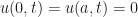
We can see how the behavior of temperature and quantum waves compare. We will consider the sourceless 1-D case for simplicity: the 1-D wire and 1-D square well. The Heat/Schrödinger equation is: Specify an initial condition () and a boundary condition at ( and ) The key to this comparison is the Wick rotation factor : By changing we can go from real to imaginary, from temperature-like to wave-like, and the strange realm in-between.
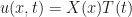
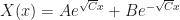
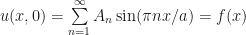
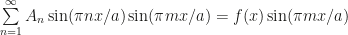
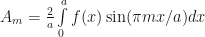
Solve using separation of variables: split time and space dependence. We then have two equations to solve: For the space component: Time component Put time and space dependence back together: There is a solution for each , so put them together for completeness: Initial condition can be written more explicitly: Use Fourier transformation to model the evolution of temperature/wave over time: In the visualizations below, the initial condition is delta function at a point between and . Both the real and imaginary components are shown. The black line is temperature-like with . Notice it flattens out and stays real. The red line is quantum wave-like with . Notice the oscillations spread out and leak into the imaginary component. The other lines, magenta, cyan and blue, are hybrids with . You can see a mix of the behaviors.
In an earlier blog entry, I discuss spacetime curvature and how it manifests as gravity in Einstein’s theory of general relativity. The elegance of a fundmental force of nature being described by the geometry of space and time has motivated people to investigate whether or not this is the case for the other fundamental forces: electromagnetism and the nuclear forces.
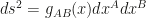
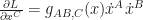
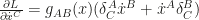
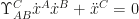
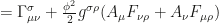
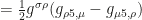
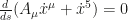
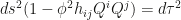
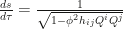
In general, for any number of dimensions, the line element of a particle’s trajectory through spacetime is: Where the indicies of and span over all dimensions of spacetime. The metric describes the curvature of spacetime. The Lagrangian is then: We can then find both sides of the Euler-Lagrange equation, which characterizes the geodesic. The left-hand side is: The right-hand side is: Put them together: Put together we get: This gives us the geodesic equation: The generalized Christoffel symbol is .
5-D Kaluza-Klein Theory It turns out that adding another spatial dimension to the spacetime metric will give us the electromagnetic force in addition to gravity. Since, we only see three spatial dimensions, this additional fourth dimension must be microscopic. This idea is known as the Kaluza-Klein theory.
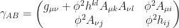
The metric of 4-D spacetime is a matrix. If we add another spatial coordinate, the metric for this 5-D spacetime becomes a matrix. This is done by concatenating a matrix with a vertical -vector, a horizontal -vector and a scalar.
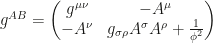
The Kaluza-Klein metric is constructed this way. The 4-D electromagnetic vector potential , which is a -vector, is concatenated to a displaced 4-D metric, along with a scalar field factor . The metric is then: The inverse of this metric is:
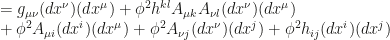
In this theory, electromagnetism arises from the spacetime curvature between 4-D spacetime and the fifth extra dimension. The 5-D line element can then be expressed in terms of the 4-D metric, the vector potential and the scalar field.
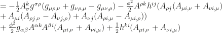
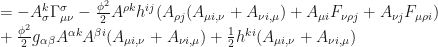
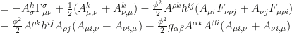
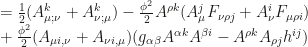
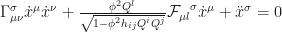
The geodesic equation can then be evaluated in terms of 4-D quantities by finding each element of the 5-D Christoffel symbol in terms of the 4-D Christoffel symbol . This allows us to view forces from this fifth dimension in more familiar 4-D quantities. Look at the 4-D subset index of the 5-D index : This can also be done for the fifth index of :
Break up the terms of the geodesic equation by dimensions: These equations give us the info we need to see how a fifth spatial dimension impacts physics. We want to evaluate the form of each Christoffel symbol factor in these equations. It is assumed that no quantities in the metric are dependent on the 5th dimensional coordinate: . This is known as the cylinder condition. We can use the definition of the Christoffel symbol to evaluate each element.
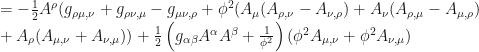
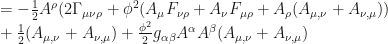
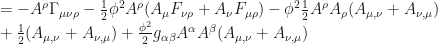
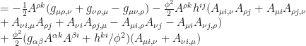
Evaluating the Christoffel Symbols Use the Kaluza-Klein metric elements to evaluate the Christoffel symbol factors. The first set of symbols are evaluated here: The first three terms here are the 4-D Christoffel symbol ! Note that the electromagnetic field strength tensor that appears here is related to the vector potential by:
Use symmetry to evaluate this one:
This next one is easy due to the cylinder condition:
This completes the first set. Onto the second set: Note the covariant derivative of the -vector potential appears:
Use symmetry again:
Use the cylinder condition again:
The Lorentz Force Emerges We can then plug in our findings into the geodesic equations. For the 4-D one we have: (equation 1)
For the 5th dimension one we have: (equation 2)
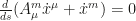
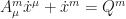
We then have a system of two equations! Equation 1 is multiplied by the vector potential to get: Summing this with equation 2 gives us: This can be expressed as a derivative with respect to proper time: Which implies the argument is constant, since the derivative is equal to zero:
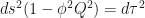
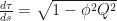
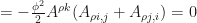
We can then uncover the nature of the scalar field by looking at the line-element again: Note the first term is the line-element, or proper time, in 4-D spacetime, and the second term looks like from above: This allows us to relate the line-elements or proper times from 5-D and 4-D spacetimes: For this derivative to be a real number, an upper bound is placed on the scalar field .
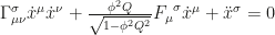
The geodesic equation 1 terms are differentiated with respect to the 5-D proper time : To see how this would appear in 4-D spacetime, translate them into 4-D proper time derivatives using the chain rule: This geodesic looks like one subject to a gravitational field and an electromagnetic field, a la the Lorentz force equation: The ratio of charge to mass is then:
You can further evaluate the Ricci tensor and Ricci scalar and get Maxwell’s equations. This unifies gravity with electromagnetism. This is a remarkable result from just adding one dimension to spacetime. There are some problems though. This theory does not predict the correct masses of particles, which means there’s something wrong with it. However, it is still compelling. The dive into this idea is what gave rise to String theory.
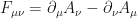
Nuclear Forces A theory that unifies gravity and electromagnetism should also unify with the nuclear forces. The weak nuclear force has already been unified with electromagnetism into what is known as the electroweak force. The strong nuclear force and electroweak force have fields with non-abelian (non-commutative) properies. We saw with electromagnetism that the field tensor is: For non-abelian fields, the field tensor is: Antisymmetry of the tensor is preserved by the structure constants being antisymmetric. The indices span the different fields that compose a force. For electroweak this maps to group elements, and for the strong force this maps to group elements.
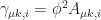
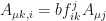
To see if we can get these forces from spacetime curvature too, start with an arbitrary number of spacetime dimensions. Here we will treat the Greek indices as 4-D spacetime, and the Latin indices as higher/extra dimensions. We can then extend the Kaluza-Klein metric : Where there are now a variety of -vector potentials , where is the index in 4-D spacetime, and is the index for extra dimensions. This implies that the different fields in the electroweak and strong force are different because they each occupy a different extra dimension. The extra dimension metric describes the curvature between the extra dimensions. The inverse of this metric is:
Like the cylinder condition from 5-D, this N-D metric has some assertions. The 4-D metric elements are not dependent on the extra dimensions: The extra dimension elements are not dependent on the extra dimensions: The extra dimension element are not dependent on 4-D spacetime: Keep in mind, the off-diagonal elements are not restricted this way. So we can have: The way the off-diagonal elements are handled here will be to facilitate the aforementioned non-abelian behavior.
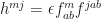
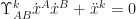
Here we can impose a gauge choice involving the structure constant by setting the associated covariant derivative equal zero: An off-diagonal field strength tensor will become handy later, and can be evaluated in terms of the structure constant: We also assert that the extra dimension metric is related to the structure constant by: The extra dimension metric can be used to raise and lower indices too: Therefore: Where is the number of extra dimensions. Therefore we have:
The Geodesic The form of the line-element can then be worked out: We then have:
The geodesic equation can be broken up the same way as before. For the 4-D terms we have: And for the extra dimension terms we have:
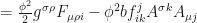
Evaluate the Christoffel symbols from the 4-D terms:
Plug these into the 4-D geodesic equation: (equation 3) Note that a symmetric and antisymmetric tensor being multiplied results in zero:
Evaluate the Christoffel symbols for the extra dimensions:
Put these together in the extra dimension geodesic:
(equation 4)
Sum equation 3 and 4 the same way we summed equations 1 and 2 for the 5-D case. Scale equation 3 by the vector potential: (equation 3)
(equation 3, scaled)
(equation 4)
The sum is then: Note the 4-D Christoffel symbols cancel out.
Unification Suppose and we get: This is a derivative with respect to proper time being equal to zero. We saw this before. We then get a set of constants for each extra dimension. equation 3 can then be written in terms of these constants:
From the line element, we can take advantage of the chain rule to put the equation in terms of 4-D proper time :
This gives us the Lorentz Force equation for charges in a non-abelian field! Where the charge mass ratio for a particle is given by: These multiple charges could be electric, weak nuclear flavors, and color charge. They are all interrelated by how the hidden extra dimensions are shaped in the metric .
A theory like this could accurately describe how all of the fundamental forces of nature may actually be the product of the same underlying phenomenon. This is the hunt for a Grand Unified Theory or a Theory of Everything. This has yet to be done successfully in physics.
Happy Holidays! Matt
All the forces emerging from spacetime curvature, but as a Christmas tree.
In my previous blog entry, I discuss Snell’s law and the refraction of light within matter. The refractive index of a substance is a metric of how much light will bend upon entering or exiting that substance. So what is the refractive index in terms of other physical variables? To address this question, we can start with Maxwell’s equations, which describe electromagnetism.
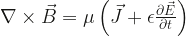
Maxwell’s equations:
Charge density is , current density is , the electric field strength is and the magnetic field strength is . Besides the charge and current densities, the other places matter enters into the equations here is in dielectric permittivity and magnetic permeability . Permittivity and permeability are related to the impedance and capacitance of substances. For instance the wave impedence of a substance is: Permittivity is a metric of how polarizable a substance is. This relates to electric dipoles within a substance. The related electric displacement field is defined by: . Permeability is a metric of how much influence an external field has on substance. This relates to the magnetic dipoles within a substance. The related Auxiliary Magnetic Field is defined as: . Keep in mind that the vacuum has permittivity and permeability as well.
If no charge or current: One remarkable result from Maxwell’s equations is that even if there are no charges or currents, , you can still have non-zero values for electric and magnetic field strength! The Maxwell’s equations without sources look like:
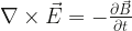
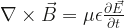
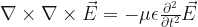
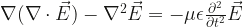
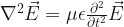
From here, we can solve for field strength . We then get partial differential equations for both fields. These are wave equations! They are identical for both the electric and magnetic field, so we only need to solve it once. These wave equations describe light! These are waves of electic and magnetic fields, hence why they are called electromagnetic waves. Note the speed of these waves will be related to the permittivity and permeability of the medium.
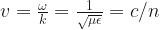
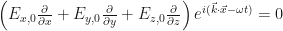
Solutions to the Wave Equations Solve for the fields’ vector components, which themselves are dependent on space and time coordinates. For example, the -component of the electric field is dependent on time and space. Assume dependence on spatial coordinates and time are seperable. Plug this into the partial differential equations to get an equation, where each term depends on one dimension of time or space. We then assert harmonic time dependence with frequency : And assert spatial symmetry, so the left hand side must have negative eigenvalues: These eigenvalues are the squared components of the wave number in terms of frequency and permittivity and permeability.
As I mentioned above, this gives the phase velocity of a light wave through a medium with permittivity and permeability . The permittivity and permeability of the vacuum gives the speed of light in a vacuum . In a general medium, we get velocities below . This is what we saw with Snell’s law! This is where the refractive index comes from! It’s dependent on the relative permeabilities and permittivities of media.
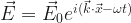
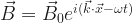
Wave Structure The -component of the electric field can be written as a product of waves in space and time. This applies to the other spatial components of the vector. Linear combinations give us sinusoidal waves and wave packets. The same solution exists for . These are oscillating waves with amplitudes of and respectively. The direction of propagation of these waves is given by the wave number vector .
Plugging these solutions into Maxwell’s equations can tell us more about the waves. Plug into the first Maxwell equation: This implies the electric field is perpendicular to the wave’s propagation: It is a transverse wave. The same can be shown for the magnetic field, using the second Maxwell equation.
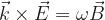
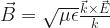
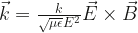
The other two Maxwell equations will show us how the fields’ vectors are oriented in space. Plug in the solutions for the electric and magnetic fields: We then evaluate the expression: This shows that the cross product between the wave number vector and electric field is proportional to the magnetic field. This implies the magnetic field is perpendicular to the electric field. The form of the magnetic field in terms of the electric field is then: The cross product of the two fields is proportional to the wave number vector. This is in the direction of propagation, and is known as the Poynting vector.
Boundary Conditions Now that we have the structure of light waves. What happens when a light wave passes from one medium to another? Imagine an electromagnetic wave passing from vacuum into water, the two media separated by a plane. When the wave starts to interact with the water, the electromagnetic field displaces charges and induces currents on the surface. This is where the electric displacement field from the displaced charges, and the auxiliary magnetic field from the induced current come into play.
Accumulated charge and current on the surface of a medium.
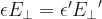
The electric field components parallel to the surface are unaffected by the plane of charges on the surface. The electric field components perpendicular to the surface are affected by the plane of charges on the surface. So there is a difference for these components. Here we need to account for the different permittivities. This manifests from the electric displacement field components perpendicular to the surface remain unchanged between media. It is the piece of the electric field from free changes. Similarly, the induced current points perpendicular to the surface, inducing a magnetic field parallel to the surface. So only the parallel components of the wave’s magnetic field are affected. This manifests from the auxiliary magnetic field components parallel to the surface remaining unchanged. This accounts for the difference in permeability. It is the piece of the magnetic field produced by currents. Perpendicular components are unaffected.
Incoming Field Orientation You can think of the wavefront of light as a ring propagating perpendularly along . The directions of and are contained within this ring, but can be oriented in any way such that and are perpendicular to each other. This orientation is the polarization of the wave.
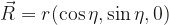
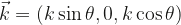
A vector bound in a ring can be defined by: Where is the angle of the vector within the ring. Tilt the z-axis towards the x-axis by . The ring is then defined by:
The direction of propagation is defined by the wave number vector. Without loss of generality, we can have the light wave propagating in a plane perpendicular to the surface of the medium: A ring tilted to be perpendicular around can be defined using the dot product:
The orientation of fields in space are then: We can check this:
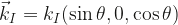
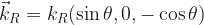
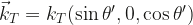
Reflecting and Refracting Some portion of the wave reflects off the surface and the rest refracts through the medium. The reflected wave can be found by flipping the coordinate of , and reflect the field vectors accordingly. The incident wave vector is: The reflected wave vector is: The transmitted or refracted wave vector is: We can check the fields of all three using the Poynting vector:
The incident fields are: The reflected fields are found by flipping over : The refracted fields are rotated from to .
The electric fields of the wave inside and outside of the medium are then: The combination of the incident and reflected field is on the outside. The refracted field is on the inside. The same applies to the magnetic fields:
Connect with Boundary Conditions We can stitch the waves together from both regions using the boundary conditions mentioned earlier. From these boundary conditions we can get a system of equations.
The first equation is from the perpendicular component of the electric field. (equation 1)
The second and third equations are from the parallel component of the electric field. (equation 2) (equation 3)
The fourth equation is from the perpendicular component of the magnetic field. The magnetic field amplitude is related to the electric field amplitude, giving us: (equation 4)
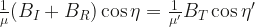
The fifth and sixth equations are from the parallel component of the magnetic field : Put into terms of electric field amplitude: (equation 5) (equation 6)
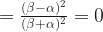
Snell’s law appears when you divide the first equation by the last equation. Or divide the fourth equation by the third.
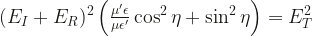
Polarization These equations can be used to figure out how much of a wave is reflected and how much is refracted. We can start by squaring equations 1 and 4, and add them together to eliminate dependence on . Add together: Do the same with equation 2 and 5: Add together: It is useful to define shorthand variables: We then have two equations:
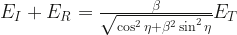
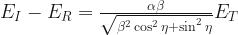
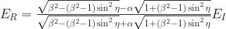
We can use these equations to solve for the field strengths. The field strengths can give us the fractions of power reflected and refracted. Solve for the reflected field and refracted field in terms of the incident field . Use these two equations to solve for reflected and refracted field strengths. Plug in in terms of :
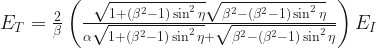
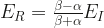
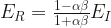
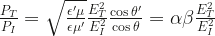
Familiar Polarization If , then . This is horizontal polarization. If then . This is vertical polarization. For each case, the equations for the refracted and reflected fields are then: for vertical polarization. For horizontal polarization: The factors here are Fresnel Coefficients, which is how much of each polarization is transmitted or reflected. The power of a wave is proportional to the square of the field strength.
The fraction of power transmitted through reflection is then: For vertical polarization: For horizontal polarization:
The fraction of power transmitted through refraction is then: For vertical polarization: For horizontal polarization:
An interesting physical consequence is the Brewster’s angle. This is where vertical polarization drops to zero. The reflected light is completely polarized horizontally. (vertical polarization) We then have: In the case where magnetic permeability is roughly the same between the media The Brewster’s angle here is the arctangent of the refractive index.
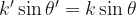
Photon Momentum Snell’s law can also be derived from quantum mechanics. The wave number vector is related to the momentum by Planck’s constant: The wave number in one medium is: The wave number in the other medium is: The ratio of these two give us the refractive index ratio: The components of the electric field parallel to surface must be equal across the boundary defined by the -plane, because the momentum of photons parallel to the surface is conserved. The component is not conserved between media, in general. This results in a deviation in angle: Therefore:
This entry is dedicated to my cousin Joe and his wife Michelle. Congratulations on tying the knot you two!
Every summer, my family would travel up to Sybil Lake in Minnesota to go fishing. When we weren’t out on the boat with our parents and Grandpa Ervin, we kids would be on the dock with our lines in the water. We’d be waiting for a bite from the same rock bass we had caught the previous day with reasonable success. I would sometimes dip my fishing rod into the water and exclaim something like “oh no, my fishing rod is bent!” It wasn’t bent though; it was the water refracting the light from the part of the rod that was submerged, making the rod appear bent. A classic prank. You can reproduce this effect with a cup of water and a straw, as seen in the picture below.
Bent straw or bent light?
Light goes from one medium (air) to another medium (water) and its behavior changes as a result. The most noticeable change here is the angle. Light comes in at an angle and is redirected to travel along a different angle by the nature of the substance it is passing through. How does this happen?
Light refracts through a medium.
On the atomic scale, the light vibrates the charges in the substance that it is passing through. These vibrating charges themselves, emit light which then interferes with the initial light, causing it to slow down and change its trajectory. The degree to which light is affected by a substance depends on how influenced it is by electric and magnetic fields. Keep in mind that light is composed of oscillating electric and magnetic fields. This phenomenon is why we have lenses and rainbows.
Fermat’s Principle It can be shown that this bent path is actually the shortest path from one medium to another. In a previous entry, I talked about the principle of least action, and how the distance between two points is not always a straight line. In this case, it can be shown to be two straight lines. In general, one medium has a refractive index of , and the other has a refractive index of . These could be water, glass, air, a vacuum, etc. The refractive index is a metric of how influenced a medium is by electric and magnetic fields.
Apply some geometry and trig to this problem.
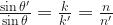
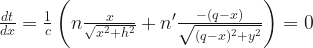
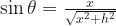
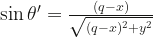
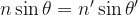
To show how this bent path between media minimizes the action, we break down the problem using geometry to parameterize the path taken by the light by a distance variable . The light will go from point A to point B, but we want to minimize the amount of time it takes to do so. The time it takes to go from A to B is the distance traveled above the water , divided by the speed above the water , added to the distance traveled below the water , divided by the speed below the water . We can then parameterize this equation in terms of distance using geometry shown in the image above. Also the fact that the speed of light in a medium is dependent on the nature of that medium , such that . To minimize the time, we take the derivative with respect to and set it equal to zero. We then get the equation: Note that these terms are equivalent to the sines of the angles in the problem: This leaves us with the following equation: which is Snell’s law! This law shows how the angle of a light beam changes from one medium to another. There are actually a number of ways to derive this law.
Wavelength and Trig It can be shown that the wavelength of the light passing through a medium changes. This can also be shown using geometry. Copy the original image and shift it over by an arbitrary distance , so there are two light beams entering the medium in the same way. You can then imagine the wavelengths along the light beams meeting at the boundary between the two media. Where one wavelength ends at the surface, another one begins. The speed of light in a medium is related to wavelength and period time by .
Wavelength change from refraction.
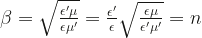
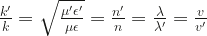
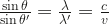
Finding the relationship between the wavelength change, the refraction angle, the incident angle then becomes a trigonometry problem. Note that in the image above, the wavelengths and distance form two triangles sharing a side, with angles : Take the ratio of these two equations (the arbitrary distance cancels out): The ratio between the speed of light from one medium to another can be thought of as an refractive index : Or in general, with two media, one with refractive index and the other with . This also gives us Snell’s law!
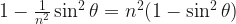
Note, there is no solution if: What does this mean? There is a critical angle where refraction stops happening. There’s no loss of generality by saying Beyond this critical angle, there is no refraction, only reflection. In general, a portion of the incoming light is refracted and a portion is reflected. Wave variables We know a wave’s speed is related to its wavelength and period by: Also note that frequency is the reciprocal of period. Another way to think about wavelength is by taking its reciprocal to get the wavenumber . (This is related to momentum in quantum mechanics by Planck’s constant ) Frequency can be scaled to angular frequency So we can express speed as:
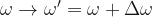
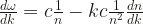
Phase and group velocity What if there is a change in frequency with respect to wavenumber ? In general, frequency is a function of wavenumber . The relationship between these two quantities depends on the nature of the media the wave is propagating through. Initially, we have a sine wave propagating at a speed of . Then the wave number starts to change from passing through a dispersive medium. In response, the frequency changes: This change transforms trig function terms: The sine wave becomes: This can also be written as: which is a convolution of two waves. One with wavelength , and the other with a wavelength of . One with the speed of as mentioned previously, and the other wave with a speed of . These quantities are known as the phase velocity and group velocity, respectively: The ratio of angular frequency and wavenumber is phase velocity and the derivative of angular frequency with respect to wavenumber is group velocity. The “groups” are thought of as envelopes or packets, wrapping the smaller wavelength wave.
Dispersion If group velocity is different from phase velocity, we get dispersion. For refraction, this means the refractive index will be dependent on wavelength. This is why we have rainbows: different colors of light will refract at different angles in water.
Light of different wavelengths (colors) refracts at different angles.
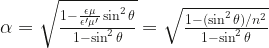
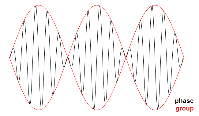
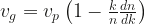
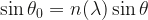
Suppose we have light in a vacuum propagating towards a medium made of matter. While in the vacuum it has a wavelength of: Once it enters the medium the wavelength becomes: From before, we know that the refractive index is the ratio of the phase velocities (or the ratio of the wavelengths). We also saw that phase velocity is the ratio between angular frequency and wavenumber. This gives us an equation relating angular frequency to wavenumber, light speed in a vacuum and the refractive index. Now suppose the refractive index is dependent on the frequency of the light . The group velocity can be found by taking the derivative. This equation can be expressed in terms of wavelength as well: Note that if the refractive index is independent of frequency that group velocity will be equivalent to phase velocity. if: We can use Snell’s law to then show angular dependence on wavelength: The incoming light is at an angle , and the refracted light is at an angle , which is dependent on the wavelength of the light. This is because the refractive index is dependent on wavelength. The way in which depends on is theorized with Cauchy’s equation: where the coefficients depend on the material. This allows rainbows to appear in the sky when sunlight refracts through raindrops.
Photo of a rainbow I took in Minnesota years ago.
If light is a wave of electric and magnetic fields, then how does it travel at the speed it does? How does a refractive index relate to these fields? How much light is reflected and how much is refracted? To address these questions, we will solve Maxwell’s equations to derive waves of light as a consequence. Maxwell’s equations: Stay tuned!
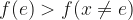
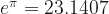
Which is greater, or ? Determine the answer without using a calculator.
Try to show which direction the inequality symbol is pointing. The solution is shown below.
The solution: Start by relating the two values with a placeholder symbol , which could be either inequality symbol or . Exponentiate both sides by This evaluates to:
Both sides can be generalized to a function of : The solution to this problem is hidden in this function. Note that . We can use this fact to write the function as:
We can use calculus to find the extrema (maximum and/or minimum) of . Take the derivative of the function: Set it equal to zero. The maximum or minimum of a function will be flat (with a slope of zero). Solve for in the resulting equation to find the extrema: So we know there is one extreme point at , but is it a max or a min?
To determine this, take the derivative of again. The second derivative is curvature. If the function curves up at the extreme point (is positive), it is a minimum. If it curves down (is negative) it is a maximum. Plug in the extreme point:
The curvature is negative! So it is a maximum. Therefore the value of is greater than the value of anywhere else along , including at : This shows that the is the greater than symbol: Therefore is larger.
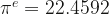
The area of a circle is proportional to the radius squared, where the proportionality constant is .
The area of a square is also proportional to the radius (or apothem) squared, where the proportionality constant is .
Circle radius and square apothem.
In general, shapes with a characteristic length have an area of the form: Where the proportionality constant depends on the shape.
So is there a way to unify circles and squares beyond stating this generic formula? How can we determine the value of for a given shape? One place to start is noting that points on a circle can be parameterized in cartesian and polar coordinates: Where any point on the -plane is related to polar coordinates by: Plugging these into the formula for a circle gives us: Which reduces to: because of the trig identity: This tells us the radius of a circle is not dependent on the angle around the center, it is a constant, which what we expect.
This can be generalized further, where instead of squaring the cartesian coordinate values of the points on a shape, we exponentiate them by : The absolute value was implied when we were squaring and , but it is made explicit here. In polar coordinates this becomes: Solving for shows us that shapes of this form have points with radial distances that depend on angle. If then we recover the circle. If we get a square, but rotated 45 degrees (diamond).
Rotated square n=1
Other values of give us shapes between circles and squares. For example, gives us a “squircle”, a shape somewhere between a circle and square.
Squircle n=4
So what are the area formulas for these shapes? This will give us the form of the proportionality constant . To do this we need to take the integral of radial distance with respect to the angle around the center of the shape. We can then plug in the general radial distance formula from the previous paragraph, giving us the form of the proportionality constant for any value of :
This integral can be evaluated approximately for a given value of by making a very small but finite number, and performing a discrete sum: where is a sufficiently large number. (Write computer code to do this sum.)
The squircle can be shown to have a proportionality constant of approximately . So the area formula for that shape is:
Below is an animation showing the shape and the approximate proportionality constant for different values of .
It is interesting how increasing the value of takes us from a star shape, to a rotated square, to a circle, to a squircle, and then gradually to a square. The proportionality constant can also be plotted against the exponent . Note that as approaches infinity, approaches , which is the proportionality constant for a square: .
I was inspired to write this entry after seeing Stand-up Maths’ video on Squircles. Check it out:
During quarantine I had some time to go through old boxes. I found a homework assignment from when I attended Professor Pran Nath’s quantum physics course in 2009. There was no accompanying solution in the box because it was a “bonus” homework from the end of the semester. So I felt like working through it now, years later. Here is my solution to that homework.
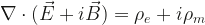
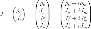
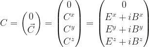
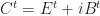
The problem asks us to show that Maxwell’s equations, in the presence of a source, can be written in a “Dirac-like” form. Where is a 4-vector of magnetic and electric field strengths, is a 4-vector of sources (electric charges, magnetic monopoles and their respective current densities), and is a 4-by-4 matrix yet to be determined.
Maxwell’s equations can be written in a more symmetric form if we suppose both electric charges and magnetic monopoles exist. We get two Gauss’ laws for electric charge and magnetic monopole densities: Ampère’s law stays the same: Faraday’s law of induction gets a current term from magnetic current, making it look more like Ampère’s law:
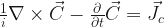
Electric and magnetic field strengths and do not add together directly. However, they can be written together as a complex field: Gauss’ laws then become: Or more compactly: Faraday’s and Ampère’s laws then become:
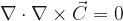
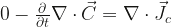
So then, Maxwell’s equations can be expressed as two equations: Because the divergence of the curl of a vector is zero, we can show that charge is conserved through a continuity equation.
Therefore: This is the continuity equation. It can also be expressed in Einstein notation: Where is a 4-vector of current and charge density elements: Similarly, the complex field strength can be expressed as a 4-vector:
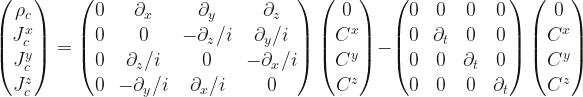
Using the two Maxwell’s equations, we can then map elements to elements: Decomposing this into 4-vector elements we get: This can be expressed as a sum of 4-by-4 matrices and derivative operations with respect to space-time:
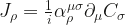
The four 4-by-4 matrices can be written as a 4-vector of matrices . This allows us to write the form of matrix mentioned above. The matrices associated with the space derivatives contain the basis elements of the Lie algebra. These are the 3-by-3 generators of rotation in 3-D space: . They also contain the 3-D unit basis vectors . The matrix associated with the time derivative contains the identity matrix in 3-D space. Note a 4th complex field could be non-zero without any effects, since the time column of is composed of all zeros, and so it would never enter Maxwell’s equations.
The Dirac-like form of Maxwell’s equations in Einstein notation is then: and since and elements occupy spacetime: This is “Dirac-like” because it looks like the Dirac equation for fermion fields. Where elements are 4-by-4 matrices multiplied by spacetime derivatives as well:
I have fond memories from grad school with Darin Baumgartel and Gregg Peim.
Gregg, myself, and Darin at Ginger Exchange years ago.
In discussions about quantum physics, you may have heard that one cannot measure both position and momentum to perfect precision. The measurement of one interferes with the measurement of another due to the wave-like nature of particles. This is known as the Heisenberg Uncertainty Principle. In this entry, I will discuss how the mathematical reasoning behind this.
In math, operations and are said to “commute” if . If they do not commute, then the order of multiplication matters: . This may seem strange if you have not worked with matrix multiplication, but you have almost certainly encountered this in real life.
An example of this kind of non-commuting algebra are rotations in 3-D space. In general, starting from the same orientation then rotating an object clockwise then top-front will give a different final configuration than rotating it top-front then clockwise. A collection of operations like this are known as a non-abelian group. In the case of rotation in 3-D space, these rotation operations are matrix multiplication on the orientation of the object. See the figures below.
Rotating clockwise, then top-front.Rotating top-front, then clockwise.
This could be written as a commutator: the general definition of which is:
Position and Momentum
To see that this kind of non-commuting algebra exists between position and momentum when dealing with quantum waves, we have to know the form of the operators involved. Imagine we want to measure momentum. We can apply the momentum operator on the wave function: If we want to measure both position and momentum , we arrive at: (equation 1)
If we change the order of the operators however, the result changes. This is because the momentum operator acts on the position operator as well as the wave function : (equation 2)
Taking the difference between equation 1 and 2 gives you the commutation relation between the momentum and position operators: (equation 3)
The fact that the difference is not zero is why there is an Uncertainty Principle. This is a key feature in quantum mechanics.
Statistics
The way the uncertainty principle arises from equation 3 involves some statistics. When you are measuring a quantity, you expect to get the average of all possible values. This is the expectation value .
If you are taking multiple measurements, the amount of change between different measurements is characterized by the standard deviation , or variance (standard deviation squared). In quantum mechanics, typically the angle bracket notation is used to denote an expectation value, instead of .
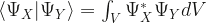
The expectation value of a measurement is the integral (or sum) over the probability density times the possible values of the measured quantity. In quantum mechanics, the probability density is determined by the wave function . We then have the operator acting on the wave function in different ways to give rise to statistical quantities.
Note, that an operator acting on a state gives another state: . This is analogous to projection of vectors. Through this particular operation, we can get the variance, which is a metric of precision. The Cauchy-Schwarz inequality on inner products of vectors applies here. This inequality relates the magnitudes of two vectors to the inner product. This same idea is carried over into what is called “Hilbert space”, where functions are vectors in infinite-dimensional space, and the inner product is the convolutional integral between two functions. (Consider another similar operator acting on state to give ). This then gives us an inequality on the variance of two variables and .
Observables
Both position and momentum are observable quantities, this means their expectation values are real numbers, and their operators are Hermitian. Hermitian operators are defined as being their own conjugate: .
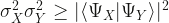
In general, the inner products of wave functions are complex numbers. The inequality we arrived at previously, then becomes:
The quantities and can be expressed in terms of and its complex conjugate. Therefore they can be expressed in terms of the inner products of the wave functions.
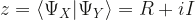
The inequality then becomes the Schrödinger uncertainty relation: If both operators and correspond to observables (both are Hermitian), then the anti-commutator is also Hermitian. This means it has a real expectation value. Therefore the first term is positive. This allows the inequality to be simplified: This allows us to get an uncertainty principle between two observable quantities and by knowing how they commute.
Proof that the anti-commutator of two Hermitian operators is also Hermitian: Therefore this is Hermitian with a real expectation value. This does not hold for the commutator however: Therefore this is not Hermitian. It is anti-Hermitian, with an imaginary expectation value.
Heisenberg Uncertainty Principle
To get the famous result, we plug in position: and momentum: Plug these into the simplified uncertainty inequality we arrived at previously: We know what the commutator is from equation 3, and we have:
It is sometimes written this way: where and The product of uncertainty in position and momentum must be greater than a positive number. Meaning you can never know both to perfect precision. Hence the name “Uncertainty Principle”. Similarly, it can be shown that time and energy have the same relationship: You can find similar uncertainty relationships when dealing with angular momentum and other observables. Not all pairs of observable quantities exhibit this limitation. The ones that do are called “complementary variables.” If you can evaluate the commutator of these, then you can get the corresponding uncertainty principle.


 .
.


 and
and 


 are idempotent


 Is the heat flow.
 Is the temperature
  gradient along the wire length
  Is the thermal conductivity of a material.
 . The heat going out of segment at
  is
is 
 ).
).

 according to the material’s mass
  .
. 
 , a total amount of heat
  flows through after a time duration
  .
.

 :
:


 differences to infinitesimal
 we have:

 (probability density) multiplied by Planck’s constant
  :
:
 divided by mass
 :
:


 )
)
 and
and  )
)
 :
:


 , so put them together for completeness:
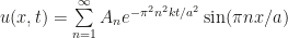


 is delta function at a point
  between
  and
and 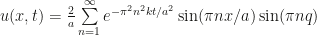
 . Notice the oscillations spread out and leak into the imaginary component.
 . You can see a mix of the behaviors.


 and
and  span over all dimensions of spacetime. The metric
  describes the curvature of spacetime. The Lagrangian is then:
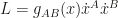


 .
.
 matrix. If we add another spatial coordinate, the metric for this 5-D spacetime becomes a
  matrix. This is done by concatenating a
  -vector, a horizontal
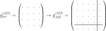
 , which is a
  . The metric is then:
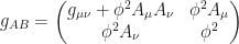

 in terms of the 4-D Christoffel symbol
  . This allows us to view forces from this fifth dimension in more familiar 4-D quantities. Look at the 4-D subset index
  of the 5-D index
  :
:


 . This is known as the cylinder condition. We can use the definition of the Christoffel symbol to evaluate each element.


 that appears here is related to the vector potential by:


 (equation 1)


 (equation 2)


 :
:
 derivatives using the chain rule:


 being antisymmetric. The indices
  span the different fields that compose a force. For electroweak this maps to
  group elements, and for the strong force this maps to
  group elements.
 :
:
 , where
  is the index in 4-D spacetime, and
  is the index for extra dimensions. This implies that the different fields in the electroweak and strong force are different because they each occupy a different extra dimension.
 describes the curvature between the extra dimensions.
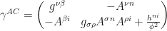


 will become handy later, and can be evaluated in terms of the structure constant:


 is the number of extra dimensions. Therefore we have:
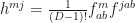


 (equation 3)


 (equation 4)
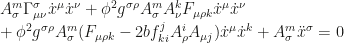 (equation 3, scaled)
 (equation 4)
 and we get:


 , current density is
  , the electric field strength is
  and the magnetic field strength is
  .
. and magnetic permeability
 .
. .
. , you can still have non-zero values for electric and magnetic field strength!

 .
.


 :
: 

 in terms of frequency


 and
and  respectively. The direction of propagation of these waves is given by the wave number vector
  .
.


 from the displaced charges, and the auxiliary magnetic field
  from the induced current come into play.


 is the polarization of the wave.

 . The ring is then defined by:


 .
.


 (equation 1)
 (equation 2)
 (equation 3)
 (equation 4)
 (equation 5)
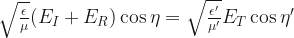 (equation 6)
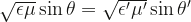


 and refracted field
  in terms of the incident field
  .
.

 , then
  . This is horizontal polarization.
 then
then  . This is vertical polarization.


 -plane, because the momentum of photons parallel to the surface is conserved.


 by the nature of the substance it is passing through. How does this happen?
 . These could be water, glass, air, a vacuum, etc. The refractive index is a metric of how influenced a medium is by electric and magnetic fields.
 , divided by the speed below the water
  .
.
 .
.

 begins. The speed of light in a medium is related to wavelength and period time by
  .
.
 :
:


 )
)

 . The relationship between these two quantities depends on the nature of the media the wave is propagating through.
 .
.


![\sin(kx - \omega(k) t) \rightarrow \sin([k + \Delta k ]x - [\omega + \Delta \omega] t)](https://s0.wp.com/latex.php?latex=%5Csin%28kx+-+%5Comega%28k%29+t%29+%5Crightarrow+%5Csin%28%5Bk+%2B+%5CDelta+k+%5Dx+-+%5B%5Comega+%2B+%5CDelta+%5Comega%5D+t%29+&bg=ffffff&fg=141412&s=1&c=20201002)

 , and the other with a wavelength of
  . One with the speed of
  .
.


 .
.


 , and the refracted light is at an angle
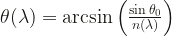
 depend on the material.
 or
or  ? Determine the answer without using a calculator.
 , which could be either inequality symbol
  or
or  .
.


 . We can use this fact to write the function as:
 .
.


 , but is it a max or a min?


 is greater than the value of
  :
:


 is the greater than symbol:
 is larger.

 .
. 


 depends on the shape.
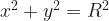


![r = \frac{R} { \sqrt[n]{|\cos\theta|^n + |\sin\theta|^n }}](https://s0.wp.com/latex.php?latex=r+%3D+%5Cfrac%7BR%7D+%7B+%5Csqrt%5Bn%5D%7B%7C%5Ccos%5Ctheta%7C%5En+%2B+%7C%5Csin%5Ctheta%7C%5En+%7D%7D&bg=ffffff&fg=141412&s=2&c=20201002)
 then we recover the circle.
 we get a square, but rotated 45 degrees (diamond).
 gives us a “squircle”, a shape somewhere between a circle and square.
 . To do this we need to take the integral of radial distance with respect to the angle around the center of the shape.

![\kappa = \frac{A}{R^2} = \frac{1}{2} \int\limits_0^{2\pi} \frac{d\theta} { \sqrt[n]{|\cos\theta|^n + |\sin\theta|^n }}](https://s0.wp.com/latex.php?latex=%5Ckappa+%3D+%5Cfrac%7BA%7D%7BR%5E2%7D+%3D+%5Cfrac%7B1%7D%7B2%7D+%5Cint%5Climits_0%5E%7B2%5Cpi%7D++%5Cfrac%7Bd%5Ctheta%7D+%7B+%5Csqrt%5Bn%5D%7B%7C%5Ccos%5Ctheta%7C%5En+%2B+%7C%5Csin%5Ctheta%7C%5En+%7D%7D+&bg=ffffff&fg=141412&s=2&c=20201002)
 a very small but finite number, and performing a discrete sum:
 squircle can be shown to have a proportionality constant of approximately
  . So the area formula for that shape is:

 approaches
  .
.

 is a 4-vector of sources (electric charges, magnetic monopoles and their respective current densities), and
  is a 4-by-4 matrix yet to be determined.


![=\frac{1}{i}\left[ -\begin{pmatrix} 0 & 0 & 0 & 0\\ 0 & i & 0 &0\\ 0 & 0 & i & 0\\ 0& 0& 0 &i\end{pmatrix} \partial_t + \begin{pmatrix} 0 & i & 0 & 0 \\ 0&0&0&0 \\ 0&0&0&-1 \\ 0&0&1&0 \end{pmatrix} \partial_x + \begin{pmatrix} 0 & 0 & i & 0 \\ 0&0&0&1\\ 0&0&0&0 \\ 0&-1&0&0 \end{pmatrix} \partial_y + \begin{pmatrix} 0 & 0 & 0& i \\ 0&0&-1&0 \\ 0&1&0&0 \\ 0&0&0&0 \end{pmatrix} \partial_z \right] \begin{pmatrix} 0 \\ C^x \\ C^y \\ C^z \end{pmatrix}](https://s0.wp.com/latex.php?latex=%3D%5Cfrac%7B1%7D%7Bi%7D%5Cleft%5B+-%5Cbegin%7Bpmatrix%7D++0+%26+0+%26+0+%26+0%5C%5C+0+%26+i+%26+0+%260%5C%5C+0+%26+0+%26+i+%26+0%5C%5C+0%26+0%26+0+%26i%5Cend%7Bpmatrix%7D+%5Cpartial_t+%2B+%5Cbegin%7Bpmatrix%7D+0+%26+i+%26+0+%26+0+%5C%5C+0%260%260%260+%5C%5C+0%260%260%26-1+%5C%5C+0%260%261%260+%5Cend%7Bpmatrix%7D+%5Cpartial_x+%2B++%5Cbegin%7Bpmatrix%7D+0+%26+0+%26+i+%26+0+%5C%5C+0%260%260%261%5C%5C+0%260%260%260+%5C%5C+0%26-1%260%260+%5Cend%7Bpmatrix%7D+%5Cpartial_y++%2B++%5Cbegin%7Bpmatrix%7D+0+%26+0+%26+0%26+i+%5C%5C+0%260%26-1%260+%5C%5C+0%261%260%260+%5C%5C+0%260%260%260+%5Cend%7Bpmatrix%7D+%5Cpartial_z+++%5Cright%5D+++%5Cbegin%7Bpmatrix%7D%C2%A00+%5C%5C%C2%A0C%5Ex+%5C%5C%C2%A0+C%5Ey+%5C%5C+C%5Ez%C2%A0%5Cend%7Bpmatrix%7D+&bg=ffffff&fg=141412&s=1&c=20201002)
 . This allows us to write the form of matrix
 Lie algebra. These are the 3-by-3 generators of rotation in 3-D space:
  . They also contain the 3-D unit basis vectors
  . The matrix associated with the time derivative contains the identity matrix in 3-D space.
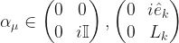
 could be non-zero without any effects, since the time column of
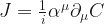
 elements are 4-by-4 matrices multiplied by spacetime derivatives as well:
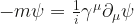

 . If they do not commute, then the order of multiplication matters:
  . This may seem strange if you have not worked with matrix multiplication, but you have almost certainly encountered this in real life.


![[\text{TopFront} ,\text{Clockwise}] \neq 0](https://s0.wp.com/latex.php?latex=%5B%5Ctext%7BTopFront%7D+%2C%5Ctext%7BClockwise%7D%5D%C2%A0+%5Cneq+0&bg=ffffff&fg=141412&s=0&c=20201002)
![[A,B] = AB-BA](https://s0.wp.com/latex.php?latex=%5BA%2CB%5D+%3D+AB-BA+&bg=ffffff&fg=141412&s=1&c=20201002)

 , we arrive at:
 (equation 1)
 acts on the position operator
  (equation 2)
![[\hat{x},\hat{p}] = \hat{x}\hat{p} - \hat{p}\hat{x} = i\hbar](https://s0.wp.com/latex.php?latex=%5B%5Chat%7Bx%7D%2C%5Chat%7Bp%7D%5D+%3D+%5Chat%7Bx%7D%5Chat%7Bp%7D+-+%5Chat%7Bp%7D%5Chat%7Bx%7D+%3D+i%5Chbar&bg=ffffff&fg=141412&s=1&c=20201002) (equation 3)
(equation 3) .
.![\mu_X = \text{E}[X] = \langle X \rangle](https://s0.wp.com/latex.php?latex=%5Cmu_X+%3D+%5Ctext%7BE%7D%5BX%5D+%3D+%5Clangle+X+%5Crangle+&bg=ffffff&fg=141412&s=1&c=20201002)
 , or variance (standard deviation squared).
![\sigma^2_X = \text{E}[(X-\mu_X)^2] = \langle (X - \langle X \rangle)^2 \rangle](https://s0.wp.com/latex.php?latex=%5Csigma%5E2_X+%3D+%5Ctext%7BE%7D%5B%28X-%5Cmu_X%29%5E2%5D+%3D+%5Clangle+%28X+-+%5Clangle+X+%5Crangle%29%5E2+%5Crangle+&bg=ffffff&fg=141412&s=1&c=20201002)

 .
.
 acting on the wave function in different ways to give rise to statistical quantities.


 . This is analogous to projection of vectors. Through this particular operation, we can get the variance, which is a metric of precision.
 acting on state
  ).
).


 .
.
 .
.


 and
and  can be expressed in terms of


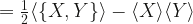


![=\frac{1}{2i} \langle [X,Y] \rangle](https://s0.wp.com/latex.php?latex=%3D%5Cfrac%7B1%7D%7B2i%7D+%5Clangle+%5BX%2CY%5D+%5Crangle+&bg=ffffff&fg=141412&s=1&c=20201002)
![\sigma_X^2 \sigma_Y^2 \geq \left( \frac{1}{2} \langle \{ X,Y \} \rangle - \langle X \rangle \langle Y \rangle \right)^2 + \left( \frac{1}{2i} \langle [X,Y] \rangle \right)^2](https://s0.wp.com/latex.php?latex=%5Csigma_X%5E2+%5Csigma_Y%5E2+%5Cgeq+%5Cleft%28+%5Cfrac%7B1%7D%7B2%7D+%5Clangle+%5C%7B+X%2CY+%5C%7D+%5Crangle+-+%5Clangle+X+%5Crangle+%5Clangle+Y+%5Crangle+%5Cright%29%5E2+%2B+%5Cleft%28+%5Cfrac%7B1%7D%7B2i%7D+%5Clangle+%5BX%2CY%5D+%5Crangle+%5Cright%29%5E2+&bg=ffffff&fg=141412&s=1&c=20201002)
 is also Hermitian. This means it has a real expectation value. Therefore the first term is positive. This allows the inequality to be simplified:
![\sigma_X^2 \sigma_Y^2 \geq \left( \frac{1}{2i} \langle [X,Y] \rangle \right)^2](https://s0.wp.com/latex.php?latex=%5Csigma_X%5E2+%5Csigma_Y%5E2+%5Cgeq+%5Cleft%28+%5Cfrac%7B1%7D%7B2i%7D+%5Clangle+%5BX%2CY%5D+%5Crangle+%5Cright%29%5E2+&bg=ffffff&fg=141412&s=1&c=20201002)


![[X,Y] = XY - YX](https://s0.wp.com/latex.php?latex=%5BX%2CY%5D+%3D+XY+-+YX+&bg=ffffff&fg=141412&s=1&c=20201002)
![[X,Y]^* = (XY-YX)^* = YX - XY = [Y,X]](https://s0.wp.com/latex.php?latex=%5BX%2CY%5D%5E%2A+%3D+%28XY-YX%29%5E%2A+%3D+YX+-+XY+%3D+%5BY%2CX%5D+&bg=ffffff&fg=141412&s=1&c=20201002)

![\sigma_x^2 \sigma_p^2 \geq \left( \frac{1}{2i} \langle [x,p] \rangle \right)^2](https://s0.wp.com/latex.php?latex=%5Csigma_x%5E2+%5Csigma_p%5E2+%5Cgeq+%5Cleft%28+%5Cfrac%7B1%7D%7B2i%7D+%5Clangle+%5Bx%2Cp%5D+%5Crangle+%5Cright%29%5E2+&bg=ffffff&fg=141412&s=1&c=20201002)


 and
and 

